Controlling XC

The exchange and correlation functional used for calculations in CASTEP can be specified in one of two main ways.

1. xc_functional
   The most straightforward is with the .param file keyword xc_functional. For example to use the PBE functional in the .param file simply use

   xc_functional : PBE
   

   There are a number of standard functionals that can be used in CASTEP with the xc_functional keyword:
   Local density approximation:
   LDA
LDA-X
LDA-C
   Generalised gradient approximations (GGA):
   PW91
PBE
PBEsol
RPBE
WC
BLYP
B86PBE
PBE_X
PBE_C
PBEsol_X
PBEsol_C
B88_X
LYP_C
   Hybrid (non-local) functionals:
   HF
SHF-LDA
PBE0
B3LYP
HSE03
HSE06
SPBE0
   Meta-GGA functionals:
   RSCAN
MS2

2. xc_definition
   The keyword xc_definition in the .param file (used instead of xc_functional) is used when you want to modify the standard behaviour of hybrid functionals, or if you want to construct your own hybrid functionals.
   The simplest use of xc_definition is to replicate that of xc_functional, for example
   

   %block xc_definition
   PBE 1.0
   %endblock xc_definition
   

   is the same as

   xc_functional : PBE
   

   The "1.0" is what weighted fraction of the functional you want, so in this case 1.0 (i.e. 100% PBE).
   Recall that hybrids are (usually) a mixture of pure (or screened) non-local Hartree-Fock exchange, some local exchange and local correlation. So you could, for example, build a functional that could be 20% Hartree Fock, 80% LDA exchange and 100% LDA correlation. You can run a CASTEP calculation with this using

   %block xc_definition
   HF 0.2
   LDA-X 0.8
   LDA-C 1.0
   %endblock xc_definition
   

Examples:
1. B3LYP Firstly you cansimply use xc_functional : B3LYP, however B3LYP is a hybrid functional consisting of a mixture of Hartree-Fock, LDA and B88 exchange, LYP and LDA correlation. This functional can be specified component by component:

%block xc_definition
LDA-X    0.08
B88_X    0.72
LYP_C    0.81
LDA-C    0.19
HF       0.20
%endblock xc_definition

Using the full specification in xc_definition makes it straightforward to adjust the various component weightings to your own specification.
There are other adjustments that can be made within the functional. For example the popular functional HSE06 contains a screened Hartree-Fock component, with a mixture of other local functionals. It can be specified component by component as

%block xc_definition
SHF 0.25
PBE 1.0
PBE_X_SR -0.25
NLXC_SCREENING_LENGTH 0.11
NLXC_SCREENING_FUNCTION ERRORFUNCTION
%endblock xc_definition

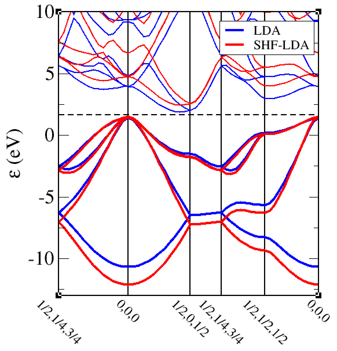
In this case we have 25% screened Hartree-Fock offsetting -25% screened PBE exchange (and 100% PBE correlation within PBE). The default HF screening is exponential, but this can be changed to an error function as shown in the block. Also the strength of the screening can be altered by the NLXC_SCREENING_LENGTH parameter (natural units).
2. Hybrid functionals are expensive calculations, much(!) more computationally intensive than (semi-)local functionals. They are often used because they are able to give much better electronic band gaps. If we do LDA and SHF-LDA band structure for silicon we can use the cell file

%block lattice_cart
2.7 2.7 0.0
2.7 0.0 2.7
0.0 2.7 2.7
%endblock lattice_cart

%block positions_frac
Si 0.00 0.00 0.00
Si 0.25 0.25 0.25
%endblock positions_frac

symmetry_generate

%block spectral_kpoint_path
W
G
X
W
L
G
%endblock spectral_kpoint_path

%block species_pot
NCP
%endblock species_pot

and then the .param file for LDA

task : spectral
spectral_task : BandStructure
xc_functional : lda

and for screened exchange,

task : spectral
spectral_task : BandStructure
xc_functional : shf-lda

If we then plot these two band structures together, the difference in results can be seen, the band gap opens from the LDA value of around 0.5eV to a more realistic 1.